Introduction
The discrete Fourier transform is a powerful tool that allows us to translate signals on a space in the time domain to a representation on the frequency domain. There are many variations of this transform, and this post will focus on what happens when we generalize the field we’re working over from the complex numbers to finite fields. We’ll cover the basics of finite fields, the definitions of the transforms, and algorithms to quickly compute them.
In general, there will be two parameters which we can modify to obtain different variations: the field and the group. The classical DFT is the Fourier transform of the cyclic group over the complex numbers.
In this article, we will consider both modifications by working over nonabelian groups such as the dihedral group and symmetric group rather than the cyclic group, and we will work over a finite field rather than the complex numbers.
The Classical Fourier Transform
The DFT is a discretization of a continuous transform that was discovered in the early 19th century by Jean-Baptiste Joseph Fourier. In particular, he used this to study PDEs that arise naturally in heat flow in a pipe. The Fourier transform takes a function in space, e.g. a distribution of heat in a linear rod, and maps the function to a frequency space as follows:
\[
\mathcal{F}: f(x) \mapsto \int_{-\infty}^{\infty} f(x)e^{-2\pi i \xi x}\,dx
\]
Often we’ll denote the function \(\mathcal{F}(f)(\xi)=\hat{f}(\xi)\). Note that the input variable is now \(\xi\) rather than \(x\), which is deliberate. \(\xi\) is said to reside in the frequency domain whereas \(x\) is in the time domain or in this case the spatial domain. Note that \(x\) is real, while the output of the transform is generally complex. One of the equations which motivated Fourier’s work is the heat equation, given by
\[
\frac{\partial u}{\partial t}=\alpha\frac{\partial^2u}{\partial x^2}.
\]
The function \(u:=u(x,t)\) depends on both space and time. For simplicity, let’s suppose we have periodic boundary conditions so that \(u(0,t)=u(L,t)\) and \(u_x(0,t)=u_x(L,t)\). Assume the ansatz that the function is separated so that \(u(x,t)=X(x)T(t)\), a product of a spatial function and a time function. This gives a pair of ODEs so that \(T’=-\alpha\lambda T\) and \(X”=-\lambda X\). For \(\lambda=(2\pi n/L)^2\), we obtain the mode
\[
u_n(x,t)=e^{2\pi i n x/L}e^{-\alpha(2\pi n/L)^2t}.
\]
Note that periodicity has forced the solution to depend on the discrete parameter \(n\).
In this case, since the function is periodic, define the Fourier transform as
\[
\hat{f}(n)=\int_0^L f(x)e^{-2\pi i n x/L}\,dx.
\]
Since the PDE is linear, a general solution can be expressed as a linear superposition of the individual solutions.
\[
u(x,t)=\sum_{n=-\infty}^{\infty}c_ne^{2\pi i n x/L}e^{-\alpha(2\pi n/L)^2t},
\]
where \(c_n=\frac{1}{L}\hat{f}(n)\).
Thus one can think of the general solution as having modes which depend on \(n\), and each mode corresponds to an eigenfunction which describes the distribution of heat in that mode, and over time the heat dissipates with exponential decay. Since we enforced periodic boundary conditions, one can imagine the heat is sloshing around inside a circular metal tube, cooling down over time.
In real applications, it is often the case that rather than having an infinitely fine, continuous set of measurements we only have a sequence of concrete measurements of some fixed number \(N\). How should the Fourier transform generalize to this case, and what types of problems would it solve?
The Discrete Fourier Transform
Imagine that we have a discrete set of measurements, a signal, which is given by \(\mathbf{x}(n):=x_n\in\mathbb{R}\). Thus, for each discrete \(n\) we have a real number. We discretize the integral using summation to obtain the discrete Fourier transform or DFT:
\[
\mathcal{F}:\mathbf{x}\mapsto
\left(\sum_{n=0}^{N-1}x_ne^{-2\pi i kn/N}\right)_{k=0}^{N-1}.
\]
That is, \(\mathcal{F}(\mathbf{x})(k):=\hat{\mathbf{x}}(k)\). In other words, given a vector \(\mathbf{x}\), we obtain a new vector with components depending on \(k\) rather than \(n\), and those components we think of as frequencies depending on the discrete parameter \(k\).
A couple things are happening here. The first thing to note is that this is a linear operator. In fact, this gives us a linear map from \(\mathbb{R}^N\rightarrow\mathbb{C}^N\). In practice, it will be useful to allow complex inputs as well as real inputs, so we obtain a linear map on the same field, \(\mathcal{F}:\mathbb{C}^N\rightarrow\mathbb{C}^N\). Using the standard basis, this transformation can be represented as an \(N\times N\) matrix.
\[
F_N=
\begin{pmatrix}
1 & 1 & 1 & \cdots & 1 \\
1 & \omega & \omega^2 & \cdots & \omega^{N-1} \\
1 & \omega^2 & \omega^4 & \cdots & \omega^{2(N-1)} \\
1 & \omega^3 & \omega^6 & \cdots & \omega^{3(N-1)} \\
\vdots & \vdots & \vdots & \ddots & \vdots \\
1 & \omega^{N-1} & \omega^{2(N-1)} & \cdots & \omega^{(N-1)(N-1)}
\end{pmatrix},
\qquad \omega=e^{-2\pi i/N}.
\]
The other important thing to note is that now that we are in the discrete realm, we could think about the index set of our vectors. It is a discrete list of numbers \(n,k\in 0,1,\ldots,N-1\). Since there are no boundary conditions a priori, it makes sense to imagine that this sequence extends to \(n=N\), but that \(x_N=x_0\), and so on so that we automatically have a periodic sequence with periodic boundary conditions.
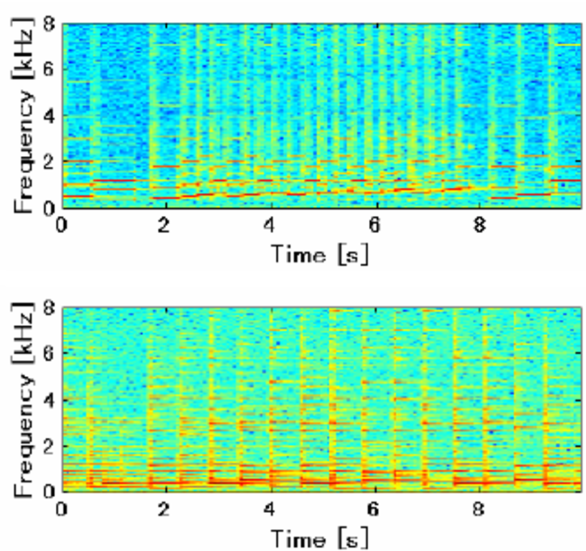
Where is this used? Well, everywhere is the answer. More specifically, it’s used in signal processing. In that case, the indexing set is taken to represent a discrete set of time measurements, and the signals are the magnitude and phase of something you’re measuring. One could measure, say, an audio signal which is sampled at some sampling rate. Then the DFT can be used to break the signal into components. This is especially useful if you’re trying to understand the pitches and frequencies contained in a musical sound. A spectrogram is obtained by taking a small piece of the time domain, performing the DFT, and then repeating in chunks to see which frequencies are approximately present for each time block. See Figure 1 to see a spectrogram for a flute and piano.
Now that we’re comfortable with the DFT, we can think a little harder about the index set. Since the signal is periodic, we have some \(x_n\) for each \(n\in\mathbb{Z}\). Since it repeats, it’s better to think of the signal as simply being defined on \(\mathbb{Z}/N\mathbb{Z}\), the cyclic group of order \(N\). A finite list of outputs depending on an input can also be thought of as a function, so now we can think of \(\mathbf{x}:\mathbb{Z}/N\mathbb{Z}\rightarrow\mathbb{C}\). Thus, \(\mathcal{F}\) is really about transforming one function defined on a cyclic group to another function defined on a cyclic group.
Let’s denote the cyclic group by \(C_N=\mathbb{Z}/N\mathbb{Z}\). We can now use the fancier notation \(\mathcal{F}:\mathbb{C}[C_N]\rightarrow\mathbb{C}[C_N]\). The algebraic object \(\mathcal{C}_N=\mathbb{C}[C_N]\) is called the group algebra of the cyclic group, and gives us a different perspective to bear on this transform. First note that \(\mathcal{C}_N\) is a vector space of dimension \(N\) over \(\mathbb{C}\). Given two elements \(a,b\) of \(\mathcal{C}_N\), we can multiply them as follows. Let \(a=\sum_i a_i\alpha^i\) and \(b=\sum_j b_j\alpha^j\). Then
\[
a\cdot b=\sum_{i,j}a_ib_j\alpha^{i+j},
\]
where again we take the indices \(i\) to be defined modulo \(N\), and \(\alpha\in C_N\) is a generator of the cyclic group. This multiplication is associative and is the reason we call this an algebra.
The next thing to notice is that every finite group has a collection of representations. Note further that \(C_N\) is an abelian group, so that its irreducible representations are one dimensional. Namely, for each \(k\) we have the map \(\rho_k:\mathbb{Z}/N\mathbb{Z}\rightarrow\mathbb{C}^{\times}\) given by \(\rho_k(n)=e^{2\pi i kn/N}\).
A representation means that the additive group law on \(\mathbb{Z}/N\mathbb{Z}\) is reflected in the multiplicative structure \(\mathbb{C}^{\times}\), so that \(\rho_k(n_0+n_1)=\rho_k(n_0)\rho_k(n_1)\). We can also recognize that \(\rho_k(n)\) is always an \(N^{th}\) root of unity. That is, \(\rho_k(n)\) lies on the unit circle \(S^1\) in the complex plane.
One dimensional representations of a group are called characters. Write \(\chi_k(n)=\rho_k(n)\). Then we can rewrite our Fourier transform as
\[
\mathcal{F}:\mathbf{x}\mapsto
\left(\sum_{n=0}^{N-1}x_n\overline{\chi_k(n)}\right)_{k=0}^{N-1}.
\]
Thus, we can now express what the DFT is in entirely new language.
Definition. The discrete Fourier transform (DFT) is the linear map from \(\mathcal{C}_N\) to \(\mathcal{C}_N\) defined by summing the components of a signal \(x_n\) against the complex conjugate of the \(k^{th}\) character \(\chi_k(n)\) over \(n\).
This immediately hints at a generalization: why not replace the cyclic group by a more complicated, nonabelian group? It turns out there is nothing stopping us, but we will have to be more careful about the definition, and work with representations which are no longer characters, i.e. their dimension is greater than one. In other words, we need to deal with representations that are matrices rather than just numbers.
The Nonabelian Fourier Transform
The simplest nonabelian group after the cyclic group is arguably the dihedral group. (There are other natural examples, such as the Heisenberg p-groups over a finite field, but the dihedral group already has representations only in dimensions 1 and 2.) The dihedral group is the symmetries of a regular polygon with \(N\) vertices in the plane, so we have both a rotation \(r\) of order \(N\), as well as a flip symmetry \(s\) of order 2. In this convention, \(D_N\) has order \(2N\).
\[
D_N=\langle r,s\mid r^N=s^2=e,\ srs^{-1}=r^{-1}\rangle.
\]
The dihedral group also has representations. One can think of a representation as a way for a group to act on a vector space. That is, given a representation \(\rho\), we can let the symmetries of the group act as \(g\cdot v=\rho(g)v\). Thus, we need \(\rho\) to map every group element \(g\) to a matrix. If the dimension of the vector space is \(d\), then this will be a \(d\times d\) matrix.
For the dihedral group, there will be representations of dimensions 1 and 2. The one dimensional characters are analogous to the characters we mentioned for the cyclic group. We can think of the two dimensional representations as \(2\times 2\) matrices which encode rotations and reflections in the plane. The behavior is different for \(N\) even and \(N\) odd.
\[
N\text{ odd}:\quad
\chi_+,\chi_-,\rho_k
\quad\text{for}\quad
k=1,\ldots,(N-1)/2,
\]
\[
N\text{ even}:\quad
\chi_1,\chi_2,\chi_3,\chi_4,\rho_k
\quad\text{for}\quad
k=1,\ldots,N/2-1.
\]
Now that we are familiar with the group algebra of a cyclic group, we can do something very straightforward: replace \(C_N\) by \(D_N\). That is, we should study the group algebra \(\mathcal{D}_N=\mathbb{C}[D_N]\). As before, we can multiply \(a,b\in\mathcal{D}_N\) via
\[
\left(\sum_g a_gg\right)
\left(\sum_h b_hh\right)
=
\sum_{g,h}a_gb_hgh.
\]
You think of these as generalizations of polynomials, where we have replaced monomials like \(x^i\) with group elements \(g\). In this generality, we can think of how the group algebra decomposes when we allow a group \(G\) to act on \(\mathbb{C}[G]\). In particular, since \(\mathbb{C}[G]\) is a ring, we can extend the action of \(G\) to an action of \(\mathbb{C}[G]\), thus we can consider the group algebra as a module over itself. The punchline is that it decomposes very nicely (over the complex numbers) into pieces which are indexed by the representations. In fact, it decomposes into pieces which are endomorphism algebras of the vector space associated to the representation. In simpler terms, these are \(d\times d\) matrix algebras. The semisimplicity statement is known as Maschke’s theorem; together with the Artin–Wedderburn theorem, it gives the decomposition we need:
Theorem (Maschke). Let \(G\) be a finite group and \(\mathbb{C}[G]\) its group algebra. Then \(\mathbb{C}[G]\) is semisimple: every \(\mathbb{C}[G]\)-module decomposes as a direct sum of irreducible submodules. Consequently, by the Artin–Wedderburn theorem, if \(\{\rho_1,\ldots,\rho_r\}\) is a complete set of pairwise non-isomorphic irreducible representations of \(G\), with \(d_i=\dim\rho_i\), then
\[
\mathbb{C}[G]\cong
\bigoplus_{i=1}^{r}\operatorname{Mat}_{d_i}(\mathbb{C})
\]as \(\mathbb{C}\)-algebras, where the isomorphism is the linear extension of \(g\mapsto(\rho_1(g),\ldots,\rho_r(g))\). In particular,
\[
|G|=\sum_{i=1}^{r}d_i^2.
\]
Thus, this theorem is telling us how to break down the group algebra using representations. There is one summand, one block, for each representation. It may be helpful to think of a representation as a sort of generalization of the notion of frequency.
Recall our earlier definition of the Fourier transform. It turns out the linear isomorphism provided by this theorem is exactly the gadget we need.
Definition. The DFT for nonabelian groups is the linear map \(\mathbb{C}[G]\rightarrow\bigoplus_\rho\operatorname{End}(V_\rho)\) given by \(\hat{f}(\rho)=\sum_g f(g)\rho(g)\).
Note that an endomorphism is a linear map from a vector space to itself. In this case, once we choose a basis, \(\operatorname{End}(V_\rho)\) is \(\operatorname{Mat}_{d\times d}\), the vector space of \(d\times d\) matrices, and \(V_\rho\) is the vector space corresponding to the representation. For the dihedral group, again, we are only getting \(1\times 1\) matrices (numbers) and \(2\times 2\) matrices.
The subtle thing to note is that \(\hat{f}(\rho)\) is a \(d\times d\) matrix, i.e. it is no longer just a number. It has \(d^2\) components. It is also important to note that there is no basis on the right hand side which is independent of our choices. For the left hand side, the group itself forms a natural basis for \(\mathbb{C}[G]\), but on the right hand side we must choose a concrete model and a basis for each representation before flattening the \(d\times d\) matrices.
Once we know the representations of a group, it is in principle possible to use this definition to compute the DFT.
This construction works for any finite group, in particular the symmetric group on \(N\) symbols, \(S_N\). The symmetric group is the group of permutations of \(N\) items \(\{1,\ldots,N\}\). It is a nonabelian group of order \(N!\). Its representation theory is much more complicated than that of the dihedral group. For now, we merely note that the representations are indexed by partitions \(\lambda\) of \(N\). The dimensions of these representations we denote by \(d_\lambda\), and they are given by an explicit formula called the hook length formula. We’ll denote the group algebra of the symmetric group by \(\mathcal{S}_N=\mathbb{C}[S_N]\).
Working Over a Finite Field
The constructions we built thus far share an interesting property, namely that they are all defined using complex numbers. However, we can ask: is there anything inherent in the complex numbers preventing us from extending these definitions to other fields of interest, namely finite fields?
If you haven’t encountered them before, finite fields are beautiful objects which have an entirely self-contained arithmetic, but only use a finite set of “numbers”. That is, one can add, subtract, multiply, and divide without leaving this finite set. The first example of a finite field, and perhaps the most useful, is the integers modulo a prime number, \(\mathbb{Z}/p\mathbb{Z}\). In a finite field, we need to divide by any nonzero number, which is what forces the modulus to be a prime. For a non-prime modulus \(m\), we could factor \(m=m_0m_1\) and then in the ring \(\mathbb{Z}/m\mathbb{Z}\), we have \(m_0m_1=m\equiv 0\text{ mod }m\).
Thus, for each prime we have a finite field. The characteristic of a finite field is \(p\), which is the smallest number such that \(p\equiv 0\) in the field. Every finite field has size a prime power \(q=p^r\) for some \(r\), and for each prime power there is a unique finite field up to isomorphism. For our purposes, the most important property is that the set of nonzero elements of the field \(\mathbb{F}_q^\times\) forms a cyclic group of order \(q-1\) (everything except zero).
We now ask what happens when we replace our favorite field \(\mathbb{C}\) with our next favorite field \(\mathbb{F}_q\)? The definition of a group algebra carries over right away, so \(\mathbb{F}_q[G]\) is still a well-defined ring. The next theorem we’d be interested in is Maschke’s theorem. It turns out that the theorem holds exactly, as long as \(p\nmid |G|\). That is, when the characteristic divides the order of the group things are nowhere near as nice, and this is the field of modular representation theory. For the remainder of the article, we’ll assume \(p\nmid |G|\). We should also note that semisimplicity alone does not guarantee that every block is a matrix algebra over \(\mathbb{F}_q\) itself: for that, \(\mathbb{F}_q\) must be a splitting field for \(G\). The hypotheses in the examples below ensure that the representations we use are defined over our chosen field.
The final ingredient we need is some notion of a root of unity. Over the complex numbers, we used \(\omega=e^{2\pi i/N}\). The property we’re after is that \(\omega^N=1\). In other words, is there a solution to \(x^N=1\) in \(\mathbb{F}_q\)? This depends on the factorization of \(x^N-1\) in characteristic \(p\), but the punchline is that a primitive \(N^{th}\) root of unity exists in \(\mathbb{F}_q\) whenever \(N\mid q-1\). If \(\gcd(N,p)=1\) but \(N\nmid q-1\), we can pass to a sufficiently large finite extension to obtain one. If \(p\mid N\), however, no finite extension of characteristic \(p\) contains a primitive \(N^{th}\) root of unity.
Subject to these hypotheses, there is nothing preventing us from replacing \(\mathbb{C}\) by \(\mathbb{F}_q\).
The Number Theoretic Transform
There are situations in which we wish to encode data rather than measure signals. In such cases, we replace a signal over the complex numbers with a list of elements in a finite field. Rather than considering functions \(\mathbb{Z}/N\mathbb{Z}\rightarrow\mathbb{C}\) as we have above, we instead consider functions \(\mathbb{Z}/N\mathbb{Z}\rightarrow\mathbb{F}_q\), and here we will also have \(N\mid q-1\).
The DFT we defined above extends naturally to this case. We can simply replace \(\omega=e^{2\pi i/N}\) with \(\tilde{\omega}\in\mathbb{F}_q\), a primitive \(N^{th}\) root of unity in the finite field. That is, \(\tilde{\omega}^N=1\) in \(\mathbb{F}_q\). Thus our Fourier transform is just
\[
\mathcal{F}:\mathbf{x}\mapsto
\left(\sum_{n=0}^{N-1}x_n\tilde{\omega}^{kn}\right)_{k=0}^{N-1}.
\]
This gives us a map \(\mathbb{F}_q^N\rightarrow\mathbb{F}_q^N\). In particular, we may choose \(q=p\) and work over the finite field \(\mathbb{Z}/p\mathbb{Z}\). Doing so yields the number theoretic transform, often abbreviated NTT.
The number theoretic transform is used heavily in cryptography. In that case, there are certain polynomial rings which look morally like \(\mathbb{F}_q[x]/(x^N-1)\), which is isomorphic to the group ring of a cyclic group over a finite field. Some lattice-based cryptosystems instead use the negacyclic ring \(R_q=\mathbb{F}_q[x]/(x^N+1)\). The choice of ring is tied to both security and efficiency; multiplication in the negacyclic ring can also be accelerated using an NTT when the field contains the appropriate roots of unity. In either case the degree is at most \(N-1\), thus we can think of the coefficients as a list of \(N\) elements of \(\mathbb{F}_q\).
Part of post-quantum cryptography is multiplying these polynomials, and we would like it to be as fast as possible. This begs the question: is there a fast version of the discrete Fourier transform, and in particular the number theoretic transform? Indeed, there is.
The Fast NTT
Again, note the usual NTT is given by \(\hat{x}_k=\sum_{n=0}^{N-1}x_n\tilde{\omega}^{nk}\). For the radix-2 algorithm, we require \(N\) to be a power of two. We split the sum into its even and odd terms as
\[
\hat{x}_k
=
\sum_{m=0}^{N/2-1}x_{2m}(\tilde{\omega}^2)^{mk}
+
\tilde{\omega}^k
\sum_{m=0}^{N/2-1}x_{2m+1}(\tilde{\omega}^2)^{mk}.
\]
Note that each sum is itself an NTT of length \(N/2\) if we recognize that the root of unity we’re using is \(\tilde{\omega}^2\) in place of \(\tilde{\omega}\). The factor \(\tilde{\omega}^k\) is called a twiddle factor. We can then proceed recursively in exactly the same manner as Cooley–Tukey.
A major difference between the DFT and NTT is that here we are working in exact arithmetic – there are no floating point errors because we’re using finite-field arithmetic.
I have implemented the underlying NTT in Rust in the ntt crate.
The FFT of the Dihedral Group Over a Finite Field
We are now in a position to combine the two generalizations we have been developing. We have replaced the cyclic group by a nonabelian group, and we have replaced the complex numbers by a finite field. Let’s start with the dihedral group, where the structure of the algorithm is especially transparent.
Recall that every element of \(D_N\) is either a rotation \(r^j\) or a reflection \(sr^j\). Thus, a function \(f:D_N\rightarrow\mathbb{F}_q\) can be written as two lists of field elements,
\[
a_j=f(r^j),
\qquad
b_j=f(sr^j),
\qquad
0\leq j<N.
\]
Assume that the characteristic \(p\) does not divide \(2N\), and that \(\mathbb{F}_q\) contains a primitive \(N^{th}\) root of unity \(\omega\). Maschke’s theorem then applies just as it did over \(\mathbb{C}\).1 In particular, the Fourier transform breaks \(\mathbb{F}_q[D_N]\) into blocks corresponding to the irreducible representations of \(D_N\). The one dimensional representations give numbers, and the two dimensional representations give \(2\times 2\) matrices.
For the two dimensional representation indexed by \(k\), we can choose
\[
\rho_k(r^j)=
\begin{pmatrix}
\omega^{kj} & 0\\
0 & \omega^{-kj}
\end{pmatrix},
\qquad
\rho_k(sr^j)=
\begin{pmatrix}
0 & \omega^{-kj}\\
\omega^{kj} & 0
\end{pmatrix}.
\]
If we plug these matrices into the definition of the nonabelian DFT, we obtain
\[
\hat{f}(\rho_k)=
\begin{pmatrix}
\displaystyle\sum_{j=0}^{N-1}a_j\omega^{kj}
&
\displaystyle\sum_{j=0}^{N-1}b_j\omega^{-kj}\\
\displaystyle\sum_{j=0}^{N-1}b_j\omega^{kj}
&
\displaystyle\sum_{j=0}^{N-1}a_j\omega^{-kj}
\end{pmatrix}.
\]
This formula is the punchline. Each entry of the matrix is an ordinary number theoretic transform of either the rotation data \(a\) or the reflection data \(b\). Frequencies with a negative exponent are already present at the corresponding index \(N-k\). Thus the nonabelian transform can be assembled from cyclic NTTs, followed by a small amount of bookkeeping which places their outputs into \(2\times 2\) matrices. The one dimensional pieces appear at the exceptional frequencies \(0\), and also \(N/2\) when \(N\) is even.
This is a satisfying example because the noncommutativity of the dihedral group does not destroy the FFT we already know. It merely changes the shape of the answer. For the cyclic group, every frequency is a number. For the dihedral group, most frequencies are \(2\times 2\) matrices. Since the cyclic transforms cost \(O(N\log N)\) operations and assembling the matrices costs only \(O(N)\), the entire dihedral transform also costs \(O(N\log N)\) rather than the \(O(N^2)\) operations required by the definition.
It also gives us fast multiplication in the group algebra. The Fourier transform turns multiplication in \(\mathbb{F}_q[D_N]\) into ordinary multiplication inside each block. We transform two elements, multiply the one dimensional blocks as numbers and the two dimensional blocks as matrices, and then apply the inverse transform. This is exactly the same pattern as polynomial multiplication using the NTT, except that “pointwise multiplication” has become blockwise matrix multiplication.
I have implemented the dihedral transform in the fft-dihedral crate. There is also a Python implementation for those who would like to experiment with the transform directly.
The FFT of the Symmetric Group Over a Finite Field
The dihedral group is a good first nonabelian example because its irreducible representations have dimension at most two. We can now ask what happens for a group whose representations are considerably more complicated. The natural next example is the symmetric group \(S_N\).
As mentioned above, the irreducible representations of \(S_N\) are indexed by partitions \(\lambda\) of \(N\). If \(\rho_\lambda\) has dimension \(d_\lambda\), then the Fourier transform of a function \(f:S_N\rightarrow\mathbb{F}_q\) contains one \(d_\lambda\times d_\lambda\) matrix for each partition:
\[
\hat{f}(\lambda)
=
\sum_{\sigma\in S_N}f(\sigma)\rho_\lambda(\sigma).
\]
We will assume the characteristic \(p\) is greater than \(N\). In particular, \(p\) does not divide \(N!\), so Maschke’s theorem applies to \(\mathbb{F}_q[S_N]\). In this range the representations we need can be constructed over the finite field, and we again obtain a decomposition.
\[
\mathbb{F}_q[S_N]
\cong
\bigoplus_{\lambda\vdash N}
\operatorname{Mat}_{d_\lambda}(\mathbb{F}_q).
\]
The dimensions still satisfy \(\sum_{\lambda\vdash N}d_\lambda^2=N!\), as they must: the matrices on the right contain exactly as many field elements as there are permutations on the left.
Of course, the definition alone does not give a fast algorithm. If we computed every matrix entry by summing over all \(N!\) permutations, we would be throwing away nearly all of the structure of the symmetric group. The relevant structure is the chain of subgroups
\[
S_1\subset S_2\subset\cdots\subset S_N.
\]
When an irreducible representation of \(S_N\) is restricted to \(S_{N-1}\), it decomposes according to a particularly clean rule: remove one box from the partition \(\lambda\) in every valid way. This is called the branching rule. Even better, each smaller representation appears at most once. The partitions therefore form a branching diagram, and the FFT proceeds recursively down this diagram.
To see the basic idea, choose representatives \(g_j\) for the cosets of \(S_{N-1}\) in \(S_N\). Any element \(f\in\mathbb{F}_q[S_N]\) can be split into \(N\) smaller pieces,
\[
f=\sum_{j=1}^{N}g_jf_j,
\qquad
f_j\in\mathbb{F}_q[S_{N-1}].
\]
We first compute the transforms of the \(f_j\) recursively. The branching rule tells us how those smaller matrix blocks sit inside a representation of \(S_N\), and multiplication by \(\rho_\lambda(g_j)\) puts them into the correct position. In this way, the transform on \(S_N\) is assembled from transforms on \(S_{N-1}\) rather than computed from scratch. Young’s seminormal representations are especially useful here because adjacent transpositions act by sparse matrices, making these assembly steps fast.
The story is more elaborate than it was for the dihedral group, but the principle is the same. We find a subgroup whose Fourier transform we already understand, separate the larger group into pieces indexed by its cosets, and use the way representations restrict to that subgroup to put the pieces back together. For the cyclic group, this recursion is the familiar even and odd split of Cooley–Tukey. For the symmetric group, it is controlled by partitions and the branching rule.
Once again, multiplication in the group algebra becomes blockwise matrix multiplication:
\[
\widehat{fg}(\lambda)
=
\hat{f}(\lambda)\hat{g}(\lambda).
\]
So even though \(\mathbb{F}_q[S_N]\) is noncommutative and has dimension \(N!\), its Fourier transform gives us the same broad recipe we have followed throughout this article: transform, multiply the frequency components, and transform back. The only difference is that the frequency components are now matrices of many different sizes, indexed by the partitions of \(N\).
I have implemented this transform in Rust in the fft-symmetric crate. A Python implementation is available as well.
Applications
Applications for the FFT of the dihedral group and symmetric group over a finite field are sparse. There is a generalization of the famous NTRU algorithm, developed in 1996 by mathematicians Jeffrey Hoffstein, Jill Pipher, and Joe Silverman, called GR-NTRU meaning group ring NTRU.2 The polynomial ring used by ordinary NTRU can be written as a cyclic group ring,
\[
\mathbb{Z}[x]/(x^N-1)
\cong
\mathbb{Z}[C_N],
\]
along with the corresponding reductions \(\mathbb{Z}_p[C_N]\) and \(\mathbb{Z}_q[C_N]\). GR-NTRU replaces the cyclic group \(C_N\) by another finite group \(G\), so that multiplication instead takes place in \(\mathbb{Z}[G]\), \(\mathbb{Z}_p[G]\), and \(\mathbb{Z}_q[G]\). When \(G=D_N\) or \(G=S_N\) and the coefficient ring is compatible with the transforms above, the dihedral or symmetric group FFT can be used to speed up this multiplication. This is the only place I know of where one might require using an FFT of the dihedral group or symmetric group to speed up multiplication. I’ve implemented GR-NTRU as a Rust crate: gr-ntru crate, as well as in Python as a gr-ntru PyPI package.
- A standard reference for Maschke’s theorem and the decomposition of group algebras is J.-P. Serre, Linear Representations of Finite Groups, Chapter 1. ↩
- T. Yasuda, X. Dahan, and K. Sakurai, “Characterizing NTRU-Variants Using Group Ring and Evaluating their Lattice Security,” IACR Cryptology ePrint Archive, Report 2015/1170 (2015),
eprint.iacr.org/2015/1170. ↩